[Deeplearning(pytorch)] 10. 오토인코더로 망가진 이미지 복원하기

본 포스팅은 “펭귄브로의 3분 딥러닝, 파이토치맛” 책 내용을 기반으로 작성되었습니다. 잘못된 내용이 있을 경우 지적해 주시면 감사드리겠습니다.

10-1. 잡음 제거 오토인코더 구현

앞서 설명한 것 처럼 오토인코더는 일종의 ‘압축’을 한다. 압축은 데이터의 특성에 우선순위를 매기고 낮은 순위의 데이터를 버린다는 뜻이다. 잡음 제거 오토인코더의 아이디어는 중요한 특징을 추출하는 오토인코더 특성을 이용하여 비교적 ‘덜 중요한 데이터’ 인 잡음을 제거하는 것이다. 코드 구조는 기본적인 오토인코더와 큰 차이는 없으며, 학습시 입력에 잡음을 더하는 방식으로 복원 능력을 강화한 것이 핵심이다.
이번 코드에서는 입력 데이터에 무작위 잡음을 더할 것이다. 무작위 잡음은 torch.randn() 함수로 만들며 입력 이미지와 같은 크기의 잡음을 만든다.

# 관련 모듈 임포트
import torch
import torchvision
import torch.nn.functional as F
from torch import nn, optim
from torchvision import transforms, datasets

import matplotlib.pyplot as plt
from mpl_toolkits.mplot3d import Axes3D
from matplotlib import cm
import numpy as np

# 하이퍼파라미터
EPOCH = 10
BATCH_SIZE = 64
USE_CUDA = torch.cuda.is_available()
DEVICE = torch.device('cuda' if USE_CUDA else 'cpu')
print('다음 기기로 학습합니다:', DEVICE)

# Fashion MNIST 학습 데이터셋 준비
trainset = datasets.FashionMNIST(
    root = './.dtaa/',
    train = True,
    download = True,
    transform = transforms.ToTensor()
)

train_loader = torch.utils.data.DataLoader(
    dataset = trainset,
    batch_size = BATCH_SIZE,
    shuffle = True,
    num_workers = 2 # 데이터 로딩하는데 서브프로세스 몇 개 사용할 것인가?
)

# 오토인코더 클래스
class Autoencoder(nn.Module):
    def __init__(self):
        super(Autoencoder, self).__init__()
        self.encoder = nn.Sequential(
            nn.Linear(28*28, 128),
            nn.ReLU(),
            nn.Linear(128, 64),
            nn.ReLU(),
            nn.Linear(64, 12),
            nn.ReLU(),
            nn.Linear(12, 3),
        )
        self.decoder = nn.Sequential(
            nn.Linear(3, 12),
            nn.ReLU(),
            nn.Linear(12, 64),
            nn.ReLU(),
            nn.Linear(64, 128),
            nn.ReLU(),
            nn.Linear(128, 28*28),
            nn.Sigmoid()
        )
    
    def forward(self, x):
        encoded = self.encoder(x)
        decoded = self.decoder(encoded)
        return encoded, decoded

# 오토인코더, 옵티마이저, 손실함수 객체 생성
autoencoder = Autoencoder().to(DEVICE)
optimizer = torch.optim.Adam(autoencoder.parameters(), lr=0.005)
criterion = nn.MSELoss()

# 노이즈 생성 함수
def add_noise(img):
    noise = torch.randn(img.size()) * 0.2
    noisy_img = img + noise
    return noisy_img

# 모델 훈련 함수
def train(autoencoder, train_loader):
    autoencoder.train()
    avg_loss = 0
    for step, (x, label) in enumerate(train_loader):
        x = add_noise(x)
        x = x.view(-1, 28*28).to(DEVICE) # 입력 데이터 = 노이즈 들어간 이미지
        y = x.view(-1, 28*28).to(DEVICE) # 라벨 데이터 = 노이즈 없는 원본 이미지

        label = label.to(DEVICE)
        encoded, decoded = autoencoder(x)

        loss = criterion(decoded, y)
        optimizer.zero_grad()
        loss.backward()
        optimizer.step()

        avg_loss += loss.item()

    return avg_loss / len(train_loader)

# 에포크 만큼 모델 훈련!
for epoch in range(1, EPOCH+1):
    loss = train(autoencoder, train_loader)
    print("[Epoch {}] loss: {}".format(epoch, loss))

# Fashion MNIST 테스트 데이터셋 준비
testset = datasets.FashionMNIST(
    root = './.data/',
    train = False,
    download = True,
    transform = transforms.ToTensor()
)

# 테스트 데이터셋에서 이미지 한장 가져옴
sample_data = testset.test_data[0].view(-1, 28*28)
sample_data = sample_data.type(torch.FloatTensor)/255.

# 테스트 데이터에 노이즈 추가하여 오토인코더 모델에 적용
original_x = sample_data[0]
noisy_x = add_noise(original_x).to(DEVICE)
_, recovered_x = autoencoder(noisy_x)


f, a = plt.subplots(1, 3, figsize=(15, 15))

# 원본 이미지, 노이즈가 첨가된 이미지, 오토인코더로 복원시킨 이미지 생성
original_img = np.reshape(original_x.to('cpu').data.numpy(), (28, 28))
noisy_img = np.reshape(noisy_x.to('cpu').data.numpy(), (28, 28))
recovered_img = np.reshape(recovered_x.to('cpu').data.numpy(), (28, 28))

# 이미지 출력
a[0].set_title('Original')
a[0].imshow(original_img, cmap='gray')

a[1].set_title('Noisy')
a[1].imshow(original_img, cmap='gray')

a[2].set_title('Recovered')
a[2].imshow(original_img, cmap='gray')

plt.show()

(결과) 다음 기기로 학습합니다: cpu
       [Epoch 1] loss: 0.07847309301593411
       [Epoch 2] loss: 0.06709331419390402
       [Epoch 3] loss: 0.06537377709217036
       [Epoch 4] loss: 0.06461306062461471
       [Epoch 5] loss: 0.06412264001744389
       [Epoch 6] loss: 0.06373336944959439
       [Epoch 7] loss: 0.06345406049159544
       [Epoch 8] loss: 0.06327535370900941
       [Epoch 9] loss: 0.06308056445105244
       [Epoch 10] loss: 0.06295464348707244

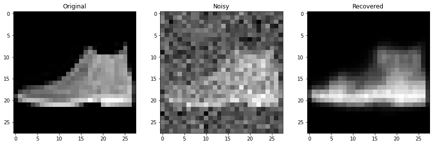
그림 10-1. 코드 결과